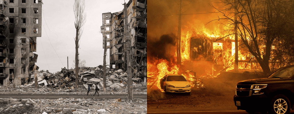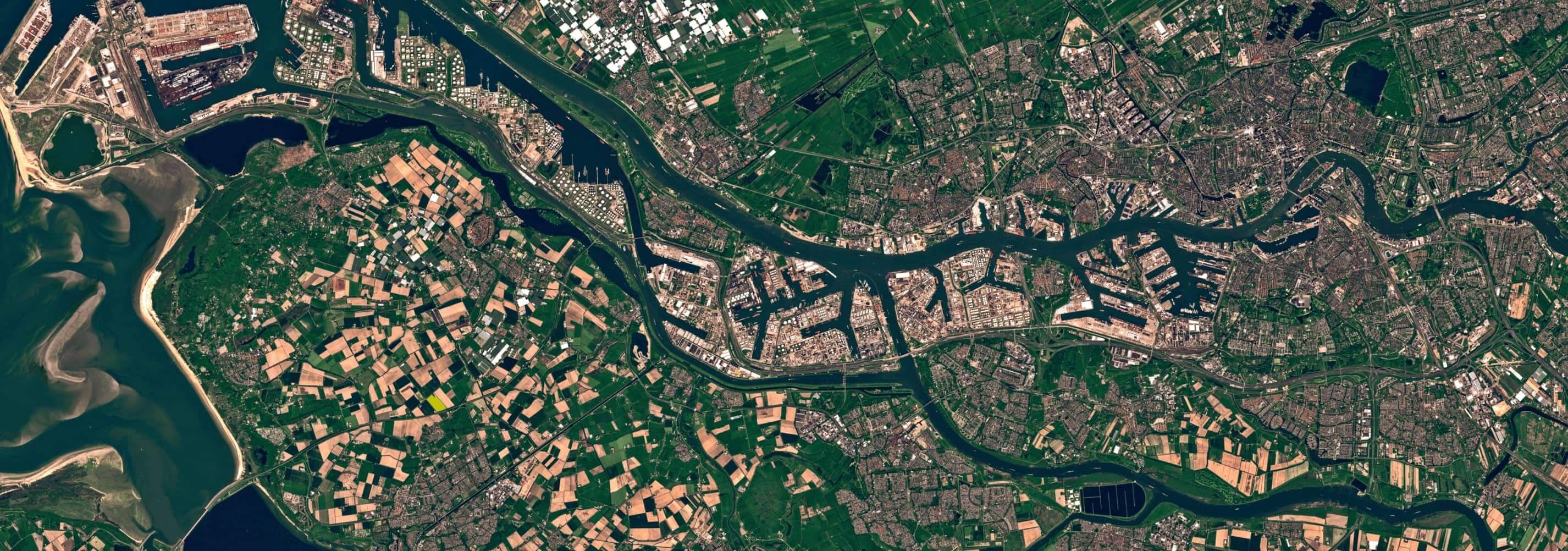
In the past decade, global conflicts and disasters accounted for 0.26% of deaths worldwide; this number is cumulative, based on the percentage of deaths from natural disasters and casualties in wars. Damage to infrastructure is one of the most significant triggers of life loss, migration, and other tragedies that can occur without a proper response. The assessment of those damages can be time-consuming and resource-intensive, especially during a disaster or shelling. To act effectively, response teams need to know the exact locations where immediate action is needed.
With the growing geospatial data analytics market and the application of deep learning, we believe that the consequences of those hazards can be reduced significantly. This article describes how modern geospatial data can increase awareness and coping ability by creating a pipeline for automated disaster control using satellite images and deep learning for damage detection.
Applying deep learning for change detection
Machine learning algorithms can help solve various problems in remote sensing, such as hyperspectral image classification, semantic 3D reconstruction and object detection. Deep learning can also be applied in terrain change detection. It is the process of spotting respective changes over time by observing the area of interest at different times. Such change detection can be applied in agriculture to observe fields’ fertility over time, monitor deforestation, and city planning.
Automated damage detection is a task that can also be approached as a supervised change detection problem. Previous studies in this field show successful applications of image segmentation in order to solve this problem. Using a pair of images that correspond to the same set of coordinates before and after a hazard (over a short period of time, assuming no structural patterns have not been changed), it is possible to identify image masks of structures in the pre-event image and then compare each mask with the post-event image.
Given that Ukraine is currently experiencing ongoing bombing from russia, we decided to test whether the model trained on natural disaster data can be used to assess damage in destroyed areas of Ukraine.
Dataset details
We have used two datasets: xView2 xBD dataset and a manually annotated dataset using Google Earth and Maxar public imagery. The first one was chosen because it is one of the largest open-source datasets for satellite damage classification. We use this dataset both for training and testing purposes. The second dataset consists of buildings’ destruction during the russo-Ukrainian War in 2014 and the 2022 russian invasion of Ukraine.
1. xView2 xBD dataset
The xBD dataset used imagery from Maxar’s Open Data program. The Open Data program provides high-resolution satellite imagery for the research community to engage in emergency planning, risk and damage assessment, monitoring of staging areas, and emergency response. It includes crowdsourced damage assessments for major natural disasters over the globe.
The dataset was manually annotated with polygons and corresponding damage scores for each building on the satellite image. It consists of 18,336 high-resolution satellite images from 6 different types of natural disasters worldwide, with over 850,000 polygons covering over 45,000 square kilometers. The data was gathered from 15 countries and contained pairs of images before (”pre”), and after (”post”) the natural disaster had occurred. All images have a resolution of 1024×1024. Also, the dataset is highly unbalanced and is skewed towards the “no-damage” class. Each pair of images contains a list of polygons (buildings) and a corresponding score from 0 to 3 based on the severity of the damage (after a disaster) for each polygon.
| Score | Label | Visual description of the structure |
|---|---|---|
| 0 | No damage | Undisturbed. No signs of water, structural damage, shingle damage or burn marks. |
| 1 | Minor damage | Buildings partially burned, water surrounding the structure, volcanic flow nearby, roof elements missing, visible cracks. |
| 2 | Major damage | Walls or the roof partially collapsed, encroaching volcanic flow, the structure is surrounded by water or mud. |
| 3 | Destroyed | The structure is scorched, completely collapsed, partially or fully covered with water or mud, no longer present. |
Figure 1: Information about the labels of the polygons in xBD dataset.
In the figure below, in left-to-right order, you may observe the satellite imagery collected before and after the disaster and the corresponding ground truth mask. The color of the buildings represents the level of destruction, where blue is “no-damage” and red is “totally-destroyed.”
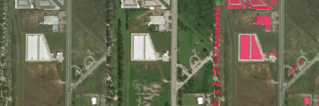
Figure 2: Example of xView Dataset
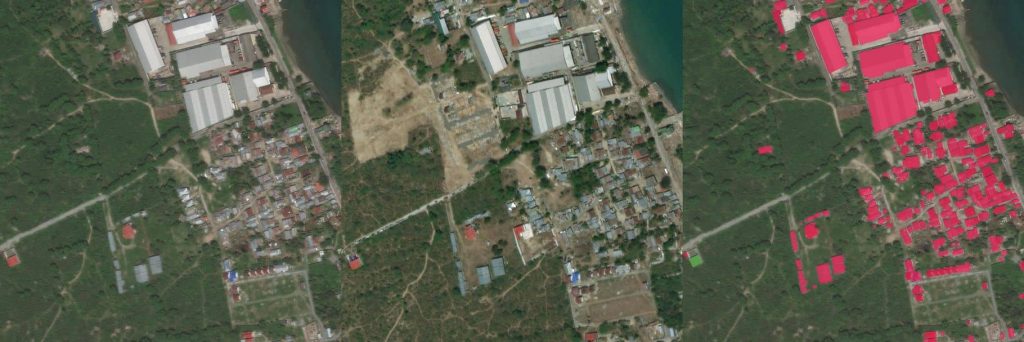
Figure 3: Example of xView Dataset
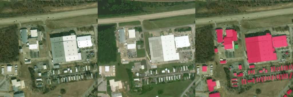
Figure 4: Example of xView Dataset
After a careful inspection of the original dataset, we observed that the borders between “no damage”-“minor damage” and “major damage”-“destroyed” are quite ambiguous and, in most cases, cannot be distinguished by eye. Moreover, in the original dataset, the structure might be damaged due to a flood event or something similar, but those damages wouldn’t be visible from a satellite top view. Thus, the decision was made to validate the approach to war damages in Ukraine by combining those classes into a single one. The resulting classes are “no-damage” and “damaged.”
2. Custom dataset: War in Ukraine 2014 & 2022
This dataset was manually selected using Google Earth imagery and publicly available imagery from Maxar. The images for each of the sources were taken during the periods of russian invasions in 2014 and 2022, respectively. In the same way as the xBD dataset, it consists of before-and-after (“pre” and ”post”) pairs of the destruction images.
The images from Google Earth have medium resolution and often are blurred or clouded. Because of that, we had to go manually city-by-city in the affected area to find not only appropriate “pre” and “post” images but also good enough in terms of visual quality. The challenge we encountered during gathering data from this source was that almost no available data is open-sourced. While comparing to Maxar ODP data, the data gathered from Google Earth has a lot lower spatial resolution, as well as the quality of the images. The data was gathered mainly from Donetsk and Luhansk regions in Ukraine.

Figure 5: Example of Google Earth pair of images from War in Ukraine 2014 (Lugansk airport 2014): Pre-event (left image) and Post-event (right image).
The images from Maxar, which are in open access, are very high-resolution but, at the same time, have great scarcity. All images have different aspect ratios and different angles of shots, which is not the ideal case, as this data doesn’t match the training dataset we have used.

Figure 6: Example of Maxar’s pair of images from War in Ukraine 2022 (East of Ukraine 2012): Pre-event (left image) and Post-event (right image).
Methodology
The primary objective of our project involves two problems: detecting buildings in images taken prior to a disaster (pre-disaster), and then classifying each building in images taken after the disaster (post-disaster) as either damaged or undamaged. We attempted to implement and test two approaches.
- In contrast to classic image segmentation tasks, our model requires two images to generate predictions.
- We only use post-damage images in order to perform instance segmentation (retrieve both building masks and the severity of impacted damages).
U-Net
U-Net is a convolutional neural network that is one of the most used in semantic segmentation. The model consists of an encoder (contraction path) and a decoder (expansion path). The encoder extracts representative feature maps of different spatial dimensions, and the decoder tries to reconstruct a semantic mask for the full resolution.
It can be used directly for multi-class segmentation on “pre” and “post” images, but this approach doesn’t perform well. Thus, we have used U-Net with different backbones and training parameters to find the best combination for the first part of our project – finding buildings on the images.
We used combined Dice Loss and Binary Focal Loss to train the network. As an optimizer, Adam optimizer was chosen with a learning rate of 0.001. The following backbones have been tested for U-Net:
- Resnet34
- Seresnext50
- Inception v3
- Efficientnet B4
Below you can observe the architecture of the Plain U-Net model:
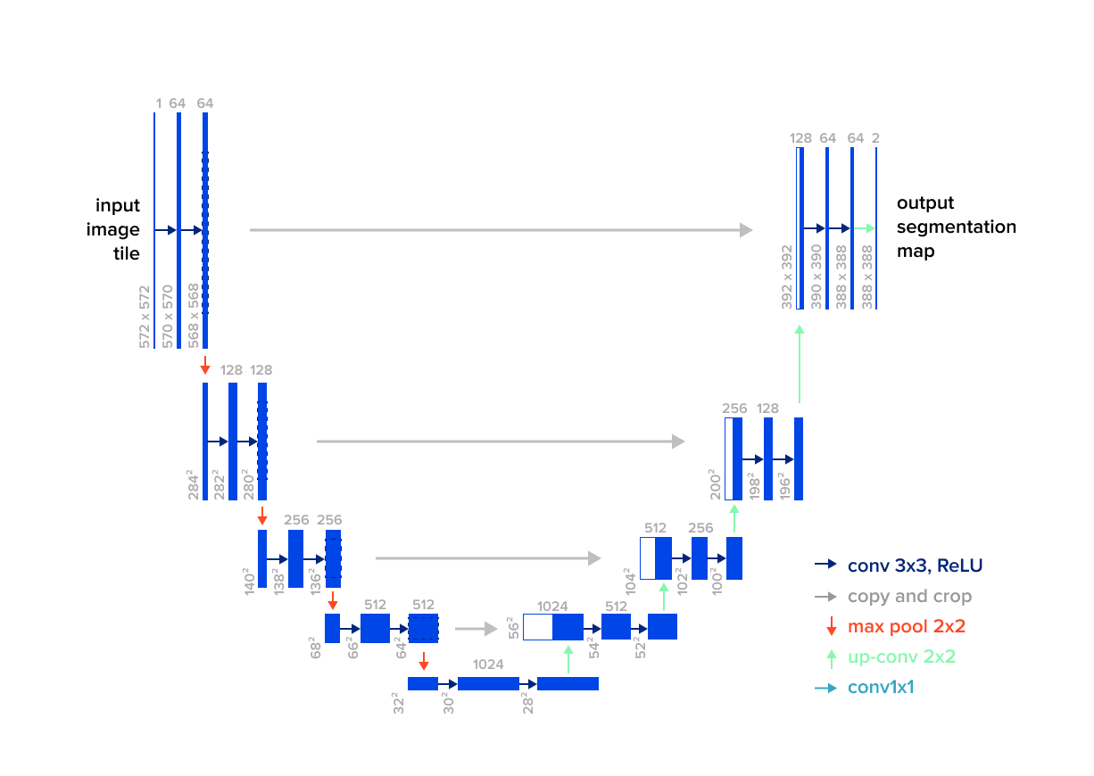
Figure 7: The architecture of the U-Net model
U-Net: 6-channels input
Another straightforward approach is to concatenate “pre” and “post” 3-channel disaster images from each pair into a single tensor with 6 channels and use it as an input to the U-Net model. The final pre+post image tensor is sent through an encoder-decoder U-Net model. The original image size is 1024×1024, but in order to increase the batch size with limited GPU capabilities, we used random image patches of 512×512 px.
Mask R-CNN
Another algorithm that was decided to use in this study is Mask R-CNN. It extends Faster R-CNN by adding a branch for predicting an object mask in parallel with the existing branch for bounding box recognition.
We used The Lovász-Softmax loss to train the network. The Adam optimizer was chosen as the optimizer, with a learning rate of 0.0001 and a weight decay of 0.0001. Similar to the previous approach, we used random image patches of 512×512 px.
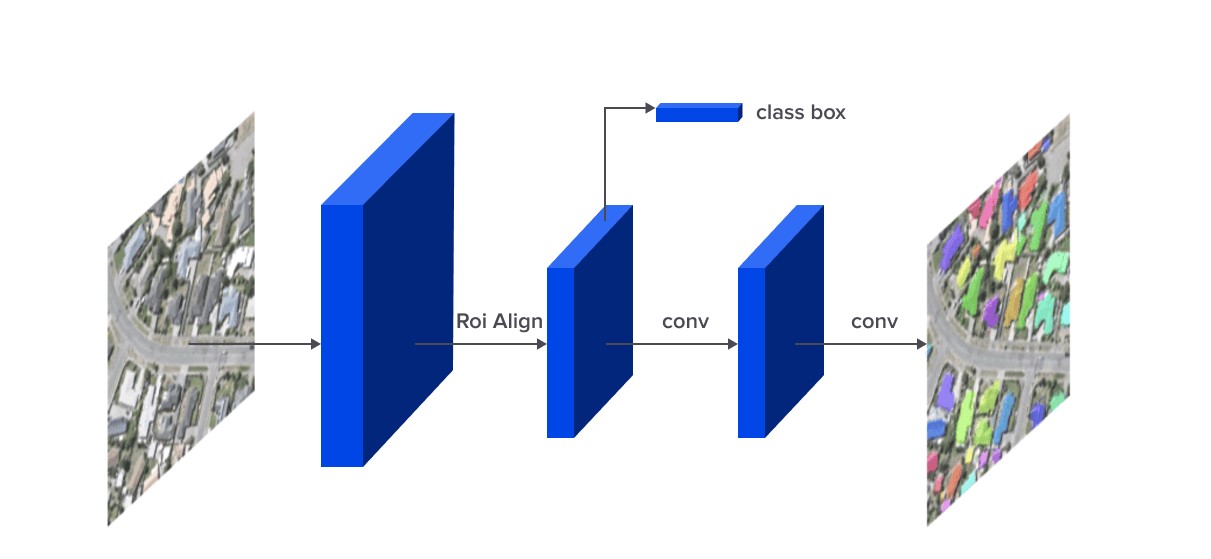
Figure 8: The Mask R-CNN framework for instance segmentation
Mask R-CNN + Mask classification
In order to compare the results of plain Mask R-CNN and make use of “pre” and “post” images, we decided to create an ensemble of Segmentation and Classification for damage assessment. In this experiment, we used Mask R-CNN as a network for “pre” image segmentation and building extraction. Afterwards, each image mask was scaled to 256×256, and Image Classification CNN was used to estimate the probability of building damage.
We used Inception v3 as a classification network with binary cross-entropy loss with Adam optimizer (learning rate of 0.0002 and a weight decay of 0.0001).
Data augmentation
Data Augmentation is a process of increasing the amount of data by changing the existing data points in a particular manner. More importantly, by using image augmentation, it is possible not only to increase the size of the dataset artificially but to make the model training process smoother and get a more generalized model that has a better performance.
After examining Google Earth Engine while constructing the dataset for war images, we observed that images could have slight color variations per channel, even when comparing samples from similar seasons (spring, summer, etc.). In order to match the possible variations, it was decided to use additional HSV augmentations alongside Random Contrast and Brightness augmentations.

Figure 9: Example of color difference on Google Earth Engine (Shyrokine, Ukraine). Left to right: Sep 2019, Sep 2020, Sep 2021
For training models in our case study, we used imgaug open-source library and applied the following image augmentations:
Spatial transformations:
- Random crop (50px on both axis)
- Random rotation (-25, +25)
- Random scaling (0.9, 1.2 on both axis)
- Random shift (-5%, +5%)
- Horizontal flip (p=0.5)
Color transformations:
- Multiply Hue and Saturation Values (0.6, 1.4 per channel) (explain why each augmentation)
- Random Contrast change
- Random Brightness change
Both Spatial and Color transformations are used within the same batch of images. Spatial transformations are applied to both pre- and post-event images in order to ensure that there is no spatial shift between a pair of images. Color transformations are applied separately to a pair of images.
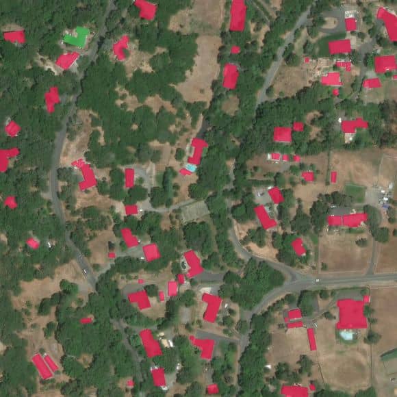
Figure 10: Original Image With Overlayed Masks

Figure 11: Example of 5 random augmentations applied
Deep learning for damage detection: experiments and results
For each pre- and post-disaster image pair, we had to produce two resulting PNG files. The first PNG file needed to contain the localization predictions (i.e., where the buildings are in the image) by having a 1 in a pixel if there is a building in the corresponding pre-disaster image and a 0 if there is no building in that pixel. The second PNG file needed to contain the damage classification predictions, where each pixel has an integer value between 1 and 2, reflecting the damage level prediction for the corresponding pixel in the post-disaster image. The F1-score of the localization and damage classification predictions was chosen as the evaluation metric.
Train/Validation split has been done based on different locations so that no overlapping images will be used for both Training and Model Validation. Moreover, a stratification based on the event type has been done (flooding, fire, hurricane, etc.) to maintain the damage nature balance.
| Approach | Train IoU (xBD) | Train F1 loc (xBD) | Train F1 cls (xBD) | Val IoU (xBD) | Val F1 loc (xBD) | Val F1 cls (xBD) | Train %Missed Buildings | Val %Missed Buildings |
|---|---|---|---|---|---|---|---|---|
| U-net (resnet34) | 0.644 | 0.739 | - | 0.616 | 0.718 | - | - | - |
| U-net (seresnext50) | 0.672 | 0.761 | - | 0.646 | 0.745 | - | - | - |
| U-net (efficientnetb4) | 0.657 | 0.758 | - | 0.636 | 0.736 | - | - | - |
| U-Net 6ch (inception v3) | 0.776 | 0.803 | 0.636 | 0.722 | 0.754 | 0.601 | 0.162 | 0.179 |
| Mask R-CNN + Clf | 0.839 | 0.872 | 0.683 | 0.814 | 0.837 | 0.671 | 0.138 | 0.142 |
| Mask R-CNN (Plain) | 0.834 | 0.861 | 0.664 | 0.801 | 0.817 | 0.657 | 0.145 | 0.161 |
Figure 12: Train/Validation (xView dataset) results
| Approach | IoU | F1 loc | F1 cls | Train %Missed Buildings |
|---|---|---|---|---|
| U-net (resnet34) | 0.582 | 0.61 | - | - |
| U-net (seresnext50) | 0.628 | 0.662 | - | - |
| U-net (efficientnetb4) | 0.614 | 0.657 | - | - |
| U-Net 6ch (inception v3) | 0.667 | 0.698 | 0.581 | 0.176 |
| Mask R-CNN + Clf | 0.738 | 0.758 | 0.614 | 0.152 |
| Mask R-CNN (Plain) | 0.725 | 0.731 | 0.603 | 0.163 |
Figure 13: Testing results (War in Ukraine)
With U-Net networks, we have been testing localization only. As we have not obtained better results than the Mask R-CNN segmentation model, we decided to skip the damage classification task for these experiments. The best results we obtained from an ensemble of Mask R-CNN as a segmentation model and Inception v3 as a Mask Classifier model. From the evaluation results above, we can see that the performance of our solution drops significantly when we use another dataset (War in Ukraine 2014 & 2022), almost 10 percent. Again, this explains the importance of balancing different satellite image sources during the training. The examples of automated damage assessment results can be seen below:
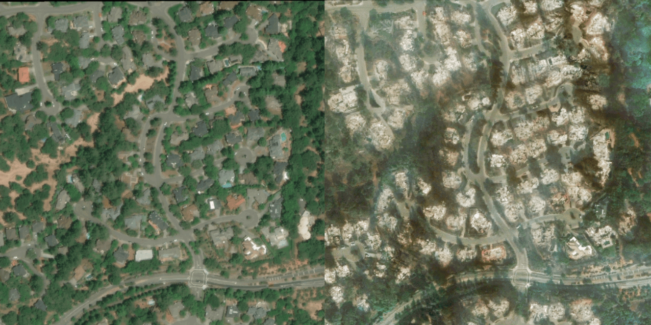
Figure 14: Example of Image “before” and “after” the event (left to right)
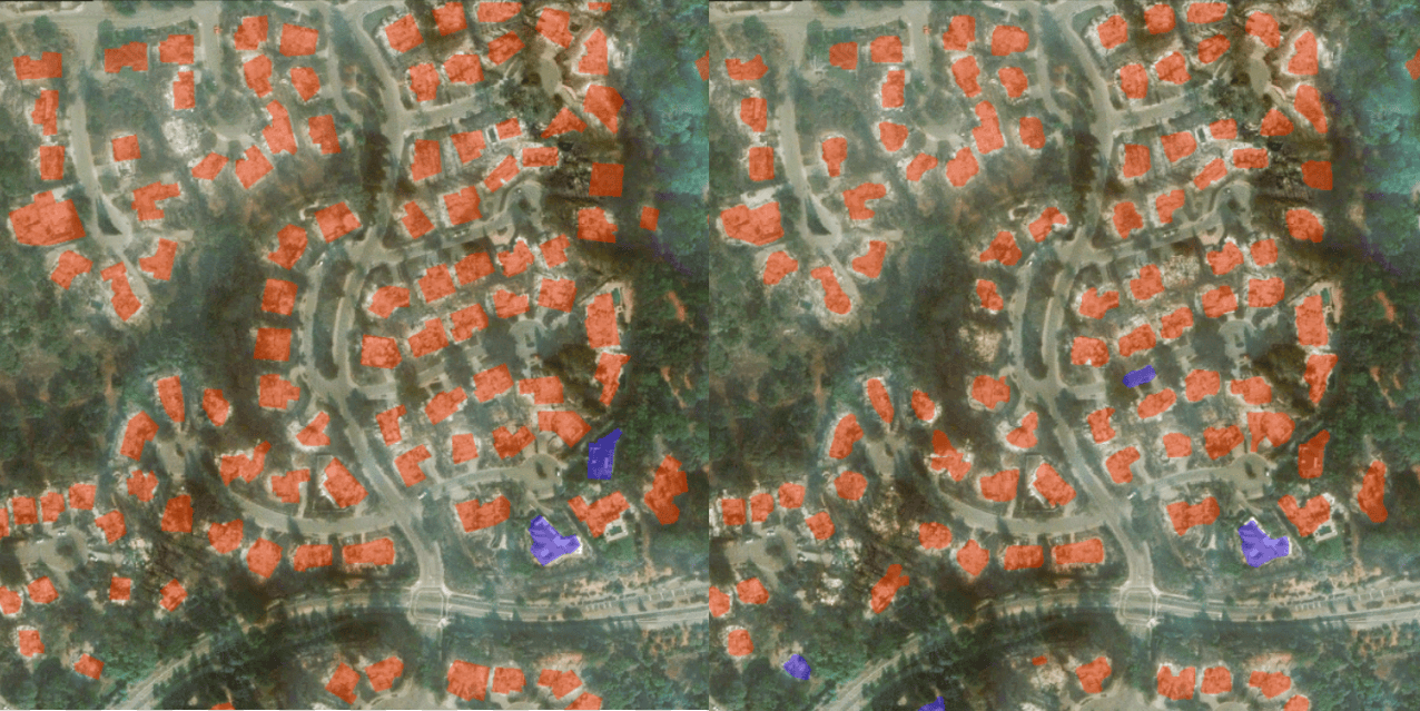
Figure 15: Example of “True” and “Predicted” damage (left to right)
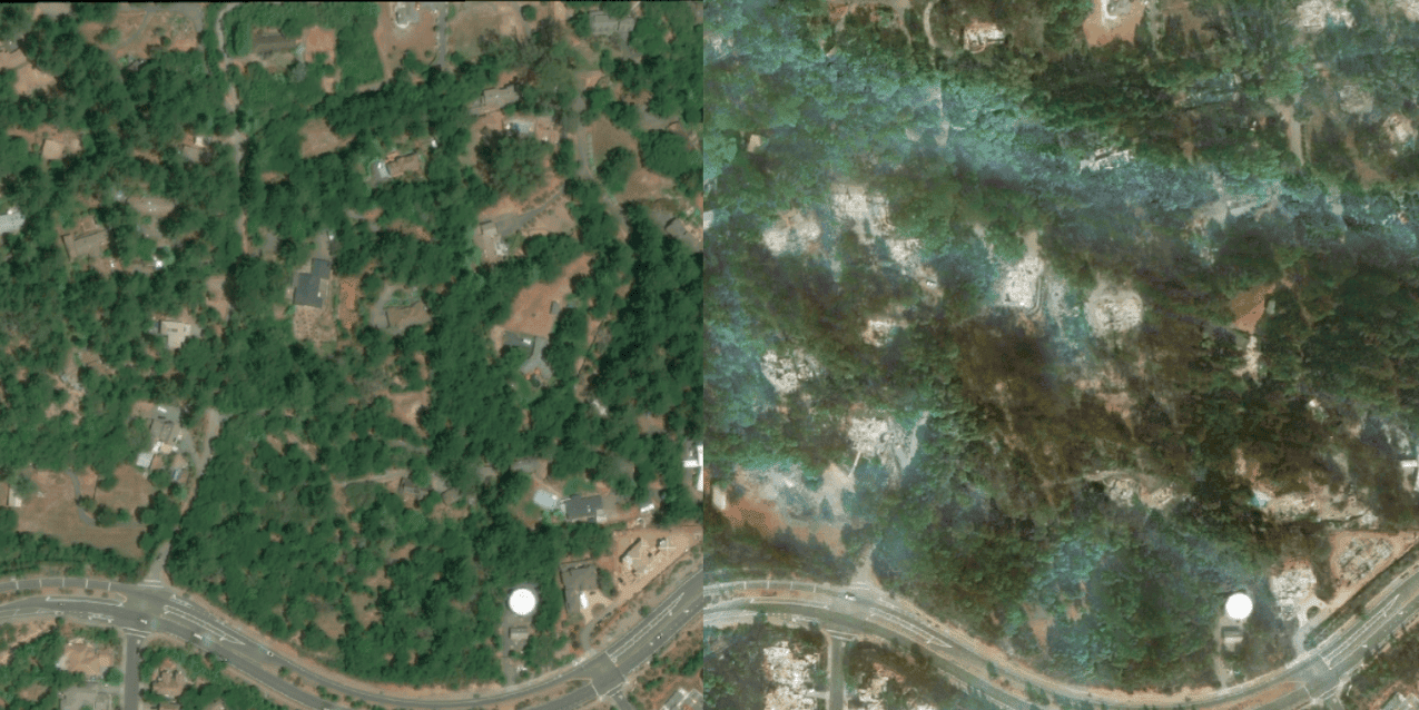
Figure 16: Example of Image “before” and “after” the event (left to right)
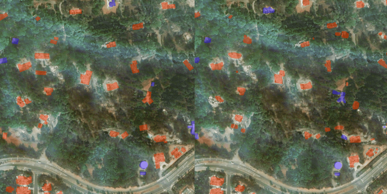
Figure 17: Example of “True” and “Predicted” damage (left to right)
The results above demonstrate the average performance of damage segmentation. It is evident that better results were achieved for images with better quality. Instead, when the model is tested on a highly-populated rural area (with a high density of buildings), its performance is actually lower. This is because the margins between individual building instances are not as well defined in such areas.
While Mask R-CNN segments structures quite accurately, there are some cases when it fails to make a correct prediction in certain cases. Two examples below show false-positive segmentation results. In the first example, we can clearly see that the pavement between two buildings is segmented as a “building” class. In the second example, it is evident that the part of the backyard is segmented as a “building,” while the original building outlines are still identified correctly. This inconsistency leads to overestimating the overall damaged area and needs to be fixed in future development.
This behavior can be seen mostly during testing the solution on the external dataset (War in Ukraine 2014 & 2022), especially when the is a satellite image of the industrial zone. This can be explained by the lack of similar images in the training dataset, as we mostly used residential areas for segmentation and damage detection.

Figure 18: Example of false-positive pavement segmentation
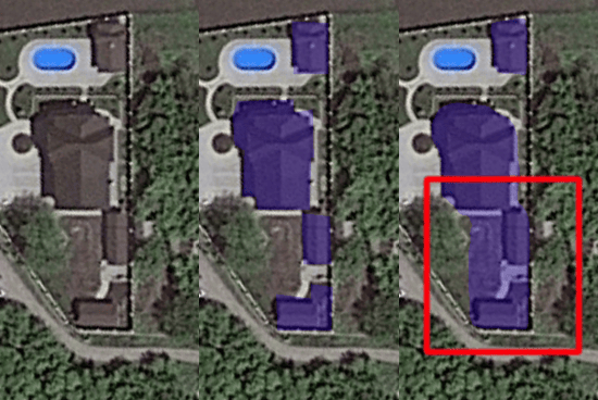
Figure 19: Example of false-positive pavement segmentation
Moreover, we can see some inconsistency during the segmentation step when there is a multi-story building in the image. The example of miss-segmentation can be seen in the example below.

The example of miss-segmentation.
Future steps
In order to improve the results and use the developed solution in a real-world scenario (e.g., automated damage estimation: War in Ukraine 2022), we would require a generalized dataset. During this work, we tried to use as many data sources as possible, and the primary purpose was to use the transfer-learning approach. We used available open-source data for training, and a custom dataset, built from different image sources (mainly Google Earth Engine) for testing and validation.
A possible solution to extend the dataset was to use building polygons extraction from Google Maps or OpenStreenMaps and use them as a ground truth mask for segmentation model training. During this step, we encountered a couple of problems, such as Google Maps satellite View is not adjusted with Google Maps vector polygons. There is a significant shift between extracted building masks and Satellite Views (see, Figure 20).

Figure 20: Google Maps Satellite view, Google Maps’ view, Extracted Building Masks from google maps (left to right)

Figure 21: Google Maps Satellite view, Google Maps’ view, Extracted Building Masks from google maps (left to right)

Figure 22: Google Maps Satellite view, Google maps view, Extracted Building Masks from google maps (left to right)
Ideally, to improve the current results for automated damage assessment in Ukraine, we would require using more data from the existing war-torn locations. Preliminary results showed that it is possible to use a transfer-learning approach in order to be able to identify war damages while performing training on natural disasters. Despite this, we have seen that even a small portion of hand-labeled domain-specific data (war damages) can improve the model results. Hence, with the actual data availability (satellite images of real battlefield locations with damaged structures), the existing results can be further enhanced.
Building a pipeline for automatic damages assessment is an essential first step in taking action for building resilient and efficient responses to both natural and anthropogenic disasters. Fast and robust damage identification can be further used in numerous risk assessments: cost assessment, migration planning, restoration assessment, etc.
By the ELEKS Data Science Office

Related insights


The breadth of knowledge and understanding that ELEKS has within its walls allows us to leverage that expertise to make superior deliverables for our customers. When you work with ELEKS, you are working with the top 1% of the aptitude and engineering excellence of the whole country.

Right from the start, we really liked ELEKS’ commitment and engagement. They came to us with their best people to try to understand our context, our business idea, and developed the first prototype with us. They were very professional and very customer oriented. I think, without ELEKS it probably would not have been possible to have such a successful product in such a short period of time.

ELEKS has been involved in the development of a number of our consumer-facing websites and mobile applications that allow our customers to easily track their shipments, get the information they need as well as stay in touch with us. We’ve appreciated the level of ELEKS’ expertise, responsiveness and attention to details.

