E-commerce Tech Trends: Reinforcement Learning for Dynamic Pricing

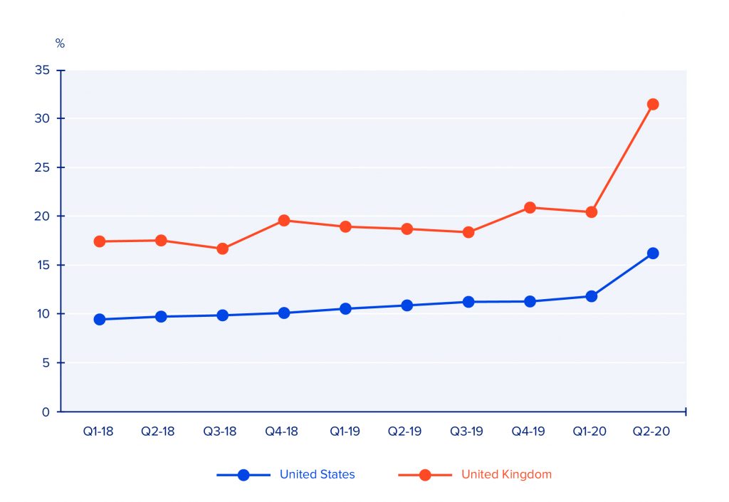
For businesses in the e-commerce, it is vital to keep pace with price movements. Overcharging for your products may result in losing customers to your competitors, while undercharging may result in less revenue. In 2019, online shopping generated $3.53 trillion in revenue for e-retailers.

Data science services and dynamic pricing, in particular, can help you determine the right price for your products and satisfy your customers’ needs. Applying reinforcement learning for dynamic pricing can help overcome dynamic pricing challenges.

What is dynamic pricing?

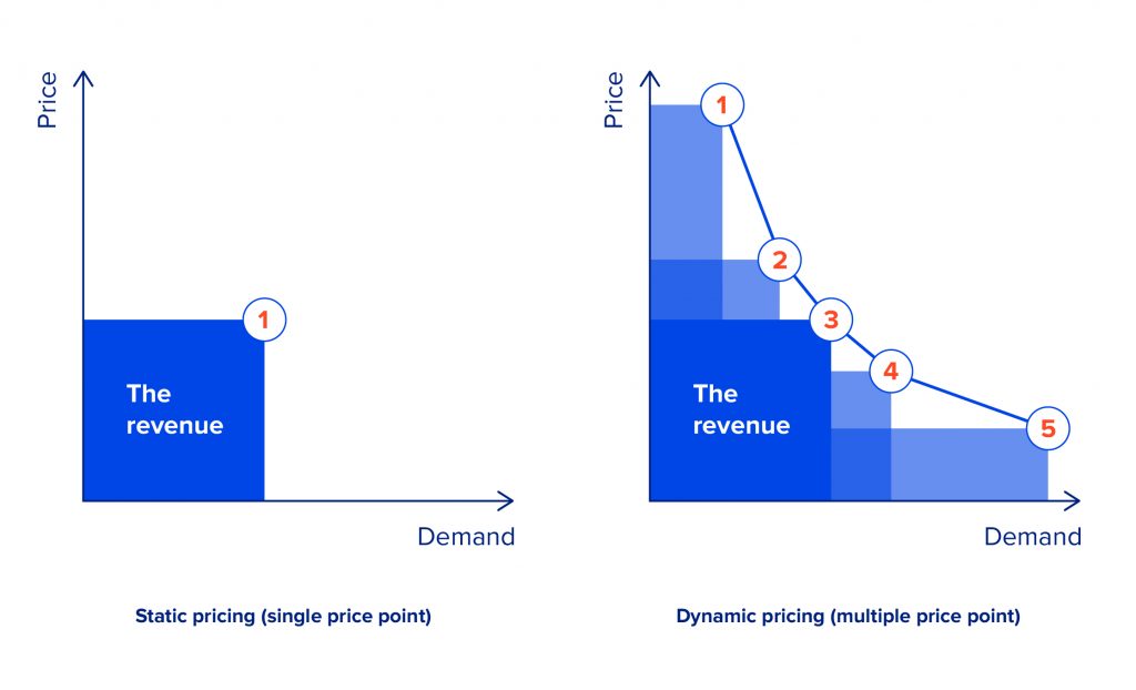
Dynamic pricing is a process of automated price adjustment for products or services in real-time to maximise income and other economic performance indicators. To define the optimal price, a dynamic pricing strategy takes into account the current market state as a basis, including the company’s previous price, changes in competitors’ prices, consumer tastes, the time range, and other exogenous factors.

Dynamic pricing strategies are applied in many business contexts and are used by airlines, train companies, concert venues, theatres, car rental companies, accommodation providers and retail companies to promptly respond to market fluctuations. For instance, Amazon monitors and changes the prices of its products every 10 minutes once the big data is updated and processed. Uber also leverages a flexible pricing strategy in case of high demand caused by bad weather or a particular event that pushes prices up.

Dynamic pricing for e-commerce: benefits

In today’s e-commerce landscape, many merchants use flexible pricing to stay competitive. Here are some key advantages of dynamic pricing in e-commerce:

• Stay ahead of competitors. Automatic monitoring of your competitors’ prices allows you to quickly adapt to the dynamic environment and gain the lead in the marketplace.
• Increase in profits. After implementing dynamic pricing, Best Buy saw an uptick in sales of 25%. By analysing the market, you can adjust the price of a product to generate more revenue. If the demand for a product is low, you can boost it by lowering the price, and if it is a peak season for a product, you can increase the price without altering your sales volume.
• Gain market insights. Continuous monitoring of the market enables you to stay aware of prevailing market trends and get insights into consumer behaviour, which can lead to better decision-making.

Dynamic pricing for e-commerce: turning challenges into success

While dynamic pricing has many advantages, the strategy itself cannot entirely eliminate the uncertainty regarding consumers’ responses to different prices. In practice, tackling this problem requires the efficient use of sales data.

Sales data is time-series data that contains prices along with respective sales and other features that could be useful in driving sales (like inventory, product seasonality, listing, etc). It is an input that a company should provide to build a dynamic pricing engine.

As it is hard to measure agent performance in real life, in this article we present an artificial example, together with theoretically optimal prices for comparison purposes. There are many different approaches for training agents to choose the optimal price for a specific time period. We start the process of building a dynamic pricing system by constructing a sales prediction model that takes as an input a market state and outputs estimated sales. This model is trained on sales data exploiting time series analysis and machine learning methods. An important note here is that the price must be in a set of input features for a prediction model. Moreover, it should have high enough feature importance.

There are two possible approaches for defining a pricing strategy when using a prognostication model:

Optimisation approach.

This is simple one-step optimisation. Using the forecasting model, you can set different prices and see how they will affect sales and income. This is a one-variable optimisation problem over a continuous interval, which is defined by a minimum and maximum price.

Since a prognostication model could be non-parametric and use non-differentiable operations, gradient-based optimisation techniques are not applicable. That is why a typical solution is to discretise a continuous interval into a countable number of possible prices and choose the price that leads to the highest income or another objective. An additional advantage of this method is that it naturally avoids the problem of falling into a local minimum.

The drawback of this approach is that it is rather greedy. In other words, it considers only income in a current timestamp rather than cumulative income over a more extended period, which is a better choice for maximisation.

Reinforcement learning (RL).

An alternative approach, and one that solves the problem of greedy decision-making, is using reinforcement learning methods. It considers associativity between the succussive pricing stages, thus being non-greedy with respect to current timestamp income, but greedy with respect to cumulative income. For example, it may be beneficial to set a lower price in the current timestamp, decreasing the possible income to get into a better market state later.

Understanding reinforcement learning basics

Reinforcement learning, or RL, is one of the three primary areas of machine learning, alongside supervised learning and unsupervised learning. Its primary task is to develop algorithms that allow agents to maximise their cumulative rewards while acting in an unknown environment. RL learns what to do (policy) and how to map situations to actions.

The idea of learning by interaction with an environment is very natural and, in some ways, is biologically inspired. As human beings, we continuously interact with the world around us, trying to maximise our reward (satisfaction, acknowledgement, money, etc.).

The environment is usually formalised by the Markov Decision Process, or MDP, a discrete-time stochastic control process. It provides a mathematical framework for modelling sequential decision making, in which the agent’s actions may influence future outcomes.

For now, we will restrict ourselves to a finite MDP. It consists of a state space S, action space A, reward space R (a subset of real numbers), and dynamics function p. Sets S, A and R are all finite. Function p defines the dynamics of the MDP.

p(s', r \mid s, a) = P(S_t=s', R_t=r|S_{t - 1}=s, A_{t - 1} = a)

\sum_{s' \in S} \sum_{r \in R} p(s', r|s, a) = 1, for all s \in S, a \in A

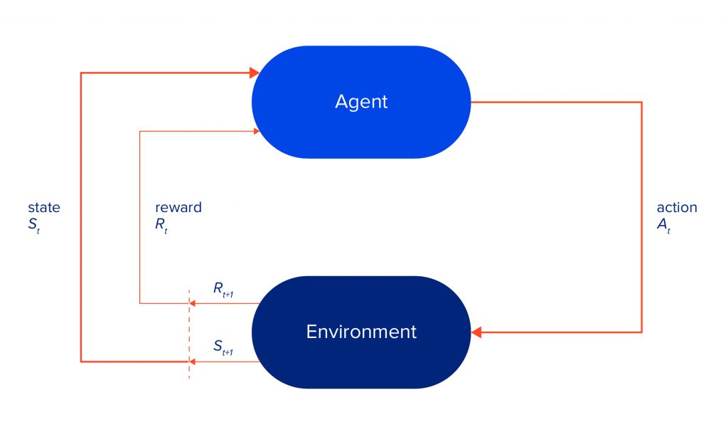
More specifically, agent and environment (MDP) interact at each time step t = 0, 1, 2, etc. The agent performs an action a, based on current state s. The MDP receives a and responds with a reward r and the next state s’. Together, they produce the following sequence:

S_0, A_0, R_1, S_1, A_1, R_2, S_2, A_2, R_3, ...

The overall process can be visualised as shown in the picture below.

RL's objective is to maximise the cumulative reward, which the agent receives in the long run (reward hypothesis). To formalise this idea, the notion of return should be defined. The return is some function of a sequence of rewards. In the case of episodic tasks (those that terminate), it can be defined as:
G_t = R_{t + 1} + R_{t + 2} + R_{t + 3} + ... + R_{T}
Policy — mapping from states to probabilities of selecting each possible action. Informally, the policy defines the rules of moving on the MDP.

\pi(a|s) = P(A_t = a|S_t=s)

Before defining an optimal policy, the notions of state-value and action value functions should be defined. Those functions are associated with a policy and show how much cumulative reward should you expect being in the state s (and taking action a):

v_{\pi}(s) = E_{\pi}[G_t | S_t=s]

q_{\pi}(s, a) = E_{\pi}[G_t | S_t=s, A_t = a]

The theory states that at least one optimal policy has the highest state-values for all states in the environment. Basically, an objective of all RL algorithms is to approximate an optimal policy.

So, why it's worth applying reinforcement learning for dynamic pricing? Read on to learn more.

Reinforcement learning for dynamic pricing

In dynamic pricing, we want an agent to set optimal prices based on market conditions. In terms of RL concepts, actions are all of the possible prices and states, market conditions, except for the current price of the product or service.

Usually, it is incredibly problematic to train an agent from an interaction with a real-world market. The reason is that an agent should gain lots of samples from an environment, which is a very time-consuming process. Also, there exists an exploration-exploitation trade-off. It means that an agent should visit a representable subset of the whole state space, trying out different actions. Consequently, an agent will act sub-optimally while training and could lose lots of money for a company.

An alternative approach is to use a simulation of the environment. Using a prognostication model, we can compute the reward (for example, income) based on the state (market conditions, except current price), and the action is the current price. So, we only need to model transitions between states. This task strongly depends on the state representation, but it tends to create a few modelling assumptions to be solved. The main drawback of the RL approach is that it is extremely hard to simulate a market accurately.

Sales data

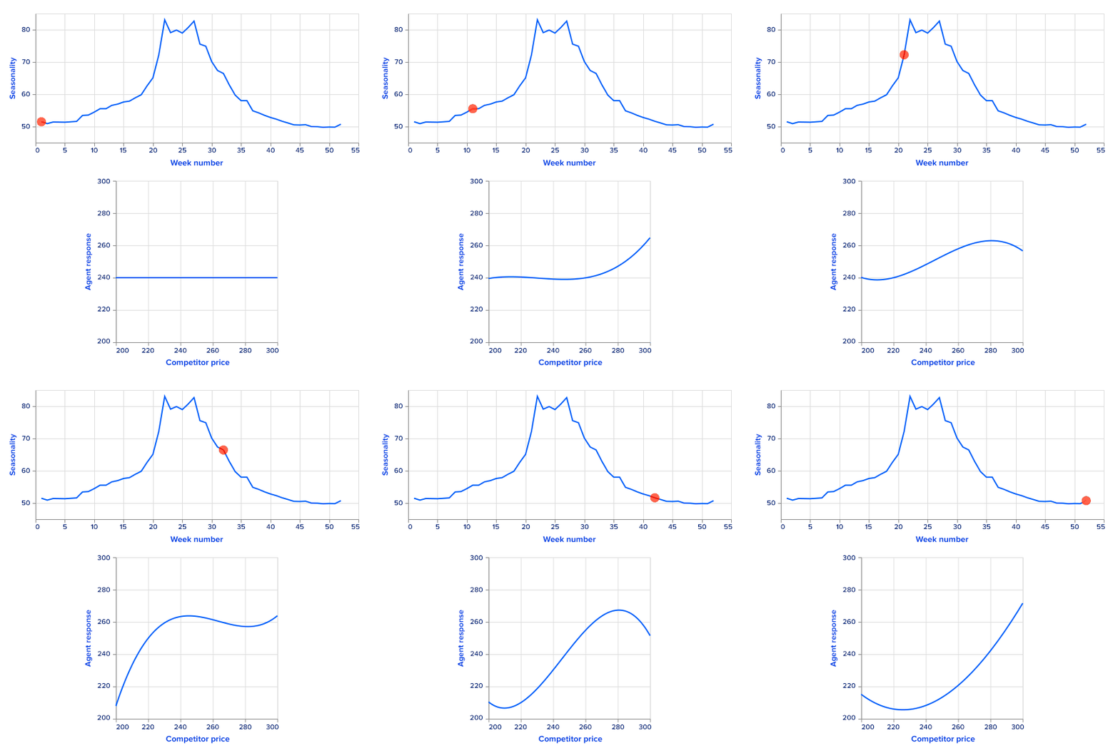
For simplicity, we use simulated sales rather than real ones. Sales data are simulated as a sum of a price-dependent component, a highly seasonal component dependent on time and a noise term. To get a seasonal component, we use the Google Trends data of a highly seasonal product – a swimming pool. Google Trends provides weekly data for over five years. There is a clear one-year seasonality in the data, so it is easy to extract it and use it as a first additive term for sales. Since this term repeats with the one year, it is a function of a week number, ranging from 0 to 52.

The second term depends on prices from the current timestamp as well as the previous timestamp to model sales. The overall formula looks like this:

sales(t, p_t, p^c_t, p_{t - 1}, p^c_{t-1}) = s(t) + f(\frac{p_t}{p^c_t}) \cdot \sigma(k \cdot f(\frac{p_{t - 1}}{p^c_{t - 1}})) + \epsilon

Here, f may be any monotonically decreasing function. The intuition is that if all other features are fixed, increasing the company’s price (either current or previous) decreases sales. On the other hand, increasing competitors’ prices leads to increased sales. The random term is sampled from a zero-mean normal distribution.

We set the function f to be linear with a negative coefficient. This allows us to analytically find a greedy policy and compare it with the RL agent's performance.

Experiments

We treat the dynamic pricing task as an episodic task with a one-year duration, consisting of 52 consecutive steps. We assume that competitors change their prices randomly.

We compare different agents by running 500 simulations and collecting cumulative rewards over 52 weeks. The graph below shows the performance of the random and greedy agents

Tabular Q-learning

Q-learning is an off-policy temporal difference control algorithm. Its main purpose is to iteratively find the action values of an optimal policy (optimal action values).

Q^*(s, a) = max_{\pi} E_{\pi}[G_t|S_t=s, A_t=a]

Using these action values, we can easily find an optimal policy. It would be any greedy policy with respect to optimal action values. The following updated formula is used:
Q(S_t, A_t) \gets Q(S_t, A_t) + \alpha [R_{t + 1} + \gamma \cdot max_a Q(S_t, a) - Q(S_t, A_t)]

The estimates converge to the optimal action values, independent of the policy used (usually epsilon-greedy with respect to the current estimates is used). This updated formula can also be treated as an iterative way of solving Bellman optimality equations.

This algorithm assumes a discrete state space and action space. Accordingly, before running this algorithm, we should discretise continuous variables into bins. The name “tabular” means that action values are stored in one huge table. Memory usage and training time grow exponentially with the increase in the number of features in the state representation, making it computationally intractable for complex environments (for example Atari games).

As we can see, this approach outperforms a random agent, but cannot outperform a greedy agent.

Deep Q-network

The deep Q-network (DQN) algorithm is based on the same idea as Tabular Q-learning. The main difference is that DQN uses a parametrised function to approximate optimal action values. More specifically, DQN uses artificial neural networks (ANNs) as approximators. Based on state representation, both convolutional neural networks and recurrent neural networks can be used.

Q(s, a; \theta) \approx Q^*(s, a)

The optimisation objective at iteration i looks as follows:

L_i(\theta_i) = E_{s, a \sim p(.)}[(y_i - Q(s, a; \theta_i)) ^ 2]

where:

y_i = E_{s' \sim \mathcal{E}}[r + \gamma max_{a'} Q(s', a'; \theta_{t - 1}) |s, a]

The behaviour distribution p is obtained by acting epsilon-greedy with respect to the previous model’s parameters.

The gradient of the objective is as follows:

\nabla_{\theta_i} L(\theta_i) = E_{s, a \sim p(.);s' \sim \mathcal{E}}[(r + \gamma max_{a'} Q(s', a'; \theta_{t - 1}) - Q(s, a; \theta_i)) \nabla_{\theta_i} Q(s, a; \theta_i)]

The loss function is optimised by stochastic gradient descent. Instead of computing a full expectation, a single-sample approximation can be used, leading to an updated Q-learning formula.

Two problems that make the optimisation process harder are correlated input data and the dependence of the target on the model’s parameters. Both problems are tackled by using an experience replay mechanism. At each step it saves a trajectory into a buffer, then instead of using a single trajectory to update parameters, a full batch sampled from a buffer is used.

With DQN you can use higher-dimensional state spaces (even images can be used). Also, it tends to be more sample-efficient than the Tabular approach. The reason is that ANNs can generalise to unseen states, even if the agent does not act from those states. On the other hand, the Tabular approach requires the whole state space to be visited. DQN is sample-efficient because it is an experience replay, which allows multiple uses of a single sample.

As we can see, DQN outperforms all other agents. Also, it was trained on a smaller number of episodes.

Policy Gradients

The policy gradients algorithm uses an entirely different idea to learn an optimal policy. Instead of learning optimal action values and moving greedily with respect to them, policy gradients directly parametrise and optimise a policy. ANNs are often used to parametrise a policy.

\pi(a|s, \theta) = P(A_t = a|S_t=s, \theta_t=\theta)

The difficulty here is that an optimisation objective, the state-value of the first state, depends on a dynamics function p, which is unknown.

J(\theta) = v_{\pi_{\theta}}(s_0)

That is why policy gradients use the fact that the gradient of the objective is an expected value of a random variable, which is approximated while acting in the environment.

\nabla J(\theta)= E_{\pi}[\sum_a \pi(a|S_t, \theta) q_{\pi}(S_t, a) \frac{\nabla \pi(a|S_t, \theta)}{\pi(a|S_t, \theta)}] = E_{\pi}[q_{\pi}(S_t, A_t) \frac{\nabla \pi(A_t|S_t, \theta)}{\pi(A_t|S_t, \theta)}] = E_{\pi}[G_t \frac{\nabla \pi(A_t|S_t, \theta)}{\pi(A_t|S_t, \theta)}]

We can subtract a baseline, which depends only on the state, from action value estimates to reduce variance. This does not affect the mean but can significantly reduce the variance, thus speeding up the learning process.

\nabla J(\theta) \propto \sum \mu(s) \sum (q_{\pi}(s, a) - b(s)) \nabla \pi(a|s, \theta)

Usually, state-value estimates are used as a baseline.

\theta_{t + 1} = \theta_t + \alpha (G_t - b(S_t)) \frac{\nabla \pi(A_t|S_t, \theta)}{\pi(A_t|S_t, \theta)}

Then stochastic gradient ascent is done using the following formula:

This method requires a lot of interaction with an environment in order to converge. 

Policy gradients outperform a greedy agent but do not perform as well as DQN. Likewise, policy gradients require far more episodes then DQN.

Please note that the real-world market environment and dependencies in it are way more complicated. This article covers a basic simulation proving that approach is working and can be applied to real data.

Reinforcement Learning for Dynamic Pricing: Conclusions

In today’s competitive environment, e-retailers face the challenge of adjusting to market changes since falling behind can mean loss of leading position and revenues. Applying reinforcement learning for dynamic pricing can become a game-changer for retail. Dynamic pricing can help retail players to stay ahead of the market, and reinforcement learning can overcome dynamic pricing challenges.